
I had the opportunity to share different classification models with a unit in the Army. I put these together to help give them what they could do as well as tell them some limitations of the models. I thought they might be useful for my students. This post is over KNN. I will have other post that discuss the other methods.
K-Nearest Neighbors
K-Nearest Neighbors (KNN) classifier will classify an unseen instance by comparing it to a “training” set.
A “training” set is a portion of data that you set aside to see how well your method of classify works. We will cover more on this later.
Once you have a new unseen instance, you compare that instance to your training set. You then decide how many neighbors (similar observations) you would like to look at (hence the “k”). The nearest neighbors are often picked by using “euclidean” distance most commonly know as straight-line distance. Here is a basic example of how this method works.
First I am going to create a simulated data set and plot it.
df = data.frame(x = c(2,2.5,1,3,3,4,4.5,4,3.5),
           y = c(1,4,2,3,4,2,1,5,5),
           c = c("success","success", "success", "success",
                 "failure", "failure", "failure", "failure",
                 "success"))
df%>%
ggplot(aes(x = x, y = y, color = c))+
geom_point(size = 5)+
labs(color = "", title = "Example K-Nearest Neighbors")+
theme(text = element_text(size = 20))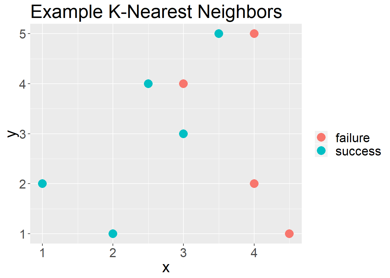
Figure 1: Example plot for using the KNN approach
In Figure 1 you see a set of points that are of two classifications, “Success” or “Failure”. Now if we had a new unseen observation, i.e. we do not know if it was a success or failure, we would compare it to the “K” nearest neighbors.
For example, in Figure 2 we have a new unseen observation.
df%>%
  ggplot(aes(x = x, y = y, color = c))+
  geom_point(size = 5)+
  labs(color = "", title = "Example K-Nearest Neighbors")+
  geom_point(aes(x = 2.5, y = 3.5), shape = 7, size = 5)+
  theme(text = element_text(size = 20))
Figure 2: Example plot of an unseen observation
If we had said we wanted to use “3” as our “k”, 2/3 of its neighbors are “success” and 1/3 of its neighbors are “failures”. We would conclude that this unseen observation is a “success”.
In Figure 3 we have another unseen observation, if we were to use “4” as our “k” we would have a 50-50 split. If we use “3” as our “k” we would predict it to be a “failure”. If we use “5” as our “k” we would predict it to b a “success”.
df%>%
  ggplot(aes(x = x, y = y, color = c))+
  geom_point(size = 5)+
  labs(color = "", title = "Example K-Nearest Neighbors")+
  geom_point(aes(x = 3.5, y = 4.5), shape = 7, size = 5)+
  theme(text = element_text(size = 20))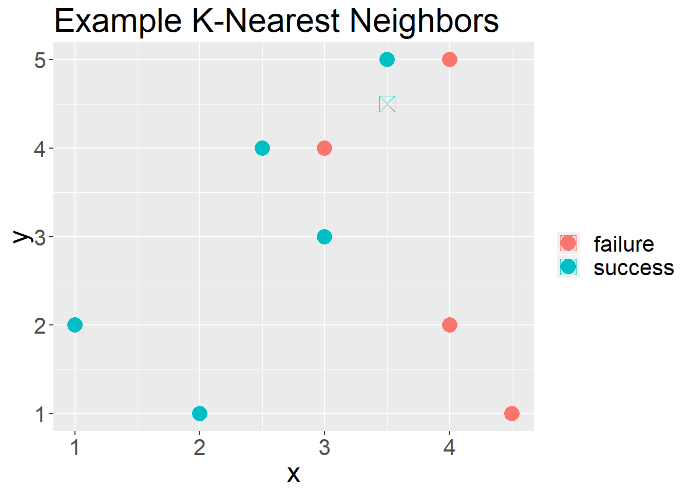
Figure 3: What about K
An example of using KNN
The following data set is know as the Iris Data set. This is a common data set used to introduce machine learning.
iris%>%
  ggplot(aes(x = Petal.Length,Petal.Width,color = Species))+
  geom_point()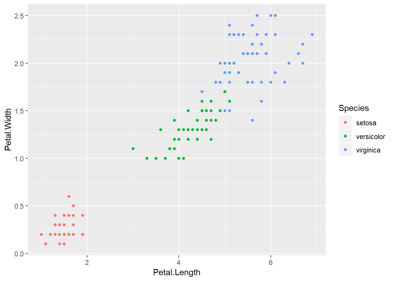
Figure 4: The Iris Data set
I am going to split my data set into two portions. The first will be my “training” set. This is what I will compare my unseen observations to. My unseen observations will by my “test” set.
iris_data = iris%>%
  mutate(id = row_number())

iris_train = iris_data%>%
  sample_frac(.8)

iris_test = iris_data%>%
  anti_join(iris_train, by = "id")
Now I will use KNN to decide how I would classify the “test” data set based on a selected “K” nearest neighbors in my “training” data set. Since, I already know the classification so I can see how well I do. To show this basic example I will be using the “caret” package. The “caret” package (short for Classification And Regression Training) contains functions to streamline the model training process for complex regression and classification problems. This is the most trusted package in R for classification problems.
test_predictions = knn3Train(train = iris_train[, 3:4], test = iris_test[, 3:4],
          cl = iris_train$Species, k = 1)
Next I will make what is known as a confusion matrix to compare my classification to the true classifications.
table(iris_test$Species, test_predictions)## test_predictions
## setosa versicolor virginica
## setosa 10 0 0
## versicolor 0 9 1
## virginica 0 0 10We did well for all the species, but got one wrong.
iris_predictions = cbind(iris_test,test_predictions)%>%
  mutate(correct = ifelse(Species == test_predictions,"yes","no"))

iris_train%>%
  ggplot(aes(x = Petal.Length, y = Petal.Width, shape = Species))+
  geom_point(size = 3)+
  geom_point(data = iris_predictions, aes(x = Petal.Length, y = Petal.Width, color = correct, shape = Species), size = 3)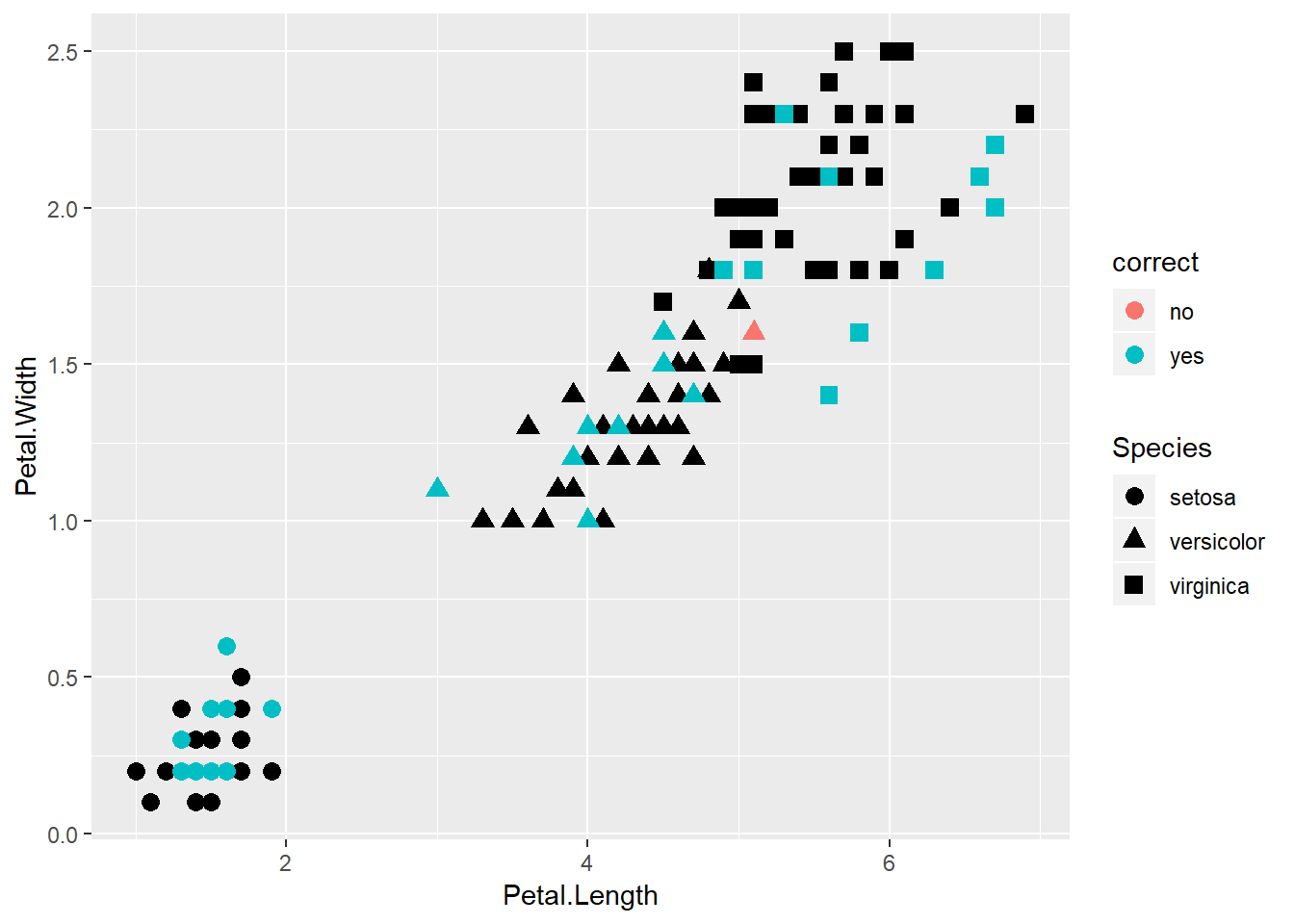
Figure 5: What was correct?
Since we only used k = 1, we missed out, but now I can move the k up to see if we do better.
test_predictions = knn3Train(train = iris_train[, 3:4], test = iris_test[, 3:4],
          cl = iris_train$Species, k = 2)

table(iris_test$Species,test_predictions)
## test_predictions
## setosa versicolor virginica
## setosa 10 0 0
## versicolor 0 9 1
## virginica 0 0 10test_predictions = knn3Train(train = iris_train[, 3:4], test = iris_test[, 3:4],
cl = iris_train$Species, k = 3)
table(iris_test$Species,test_predictions)## test_predictions
## setosa versicolor virginica
## setosa 10 0 0
## versicolor 0 9 1
## virginica 0 0 10Issues with KNN
Picking the correct K
A big issue with k-Nearest Neighbors is the choice of a suitable k. How many neighbors should you use to decide on the label of a new observation?
As you begin increase K you will see benefits in classification, but increase K to much you end up over fitting and your error will increase significantly.
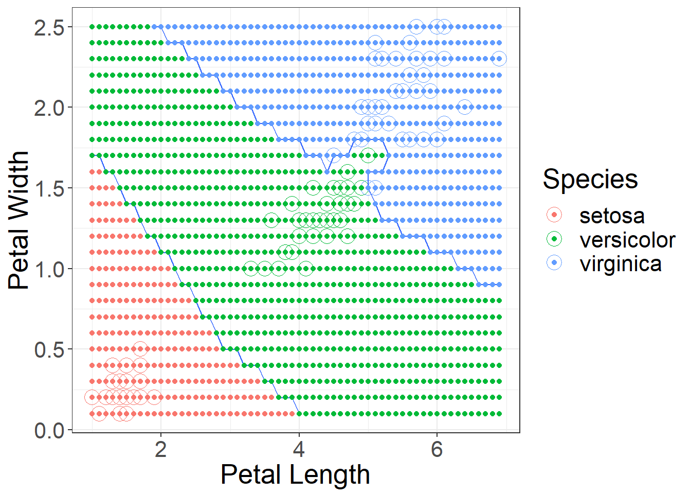
Figure 6: Using k = 1 decision boundaries
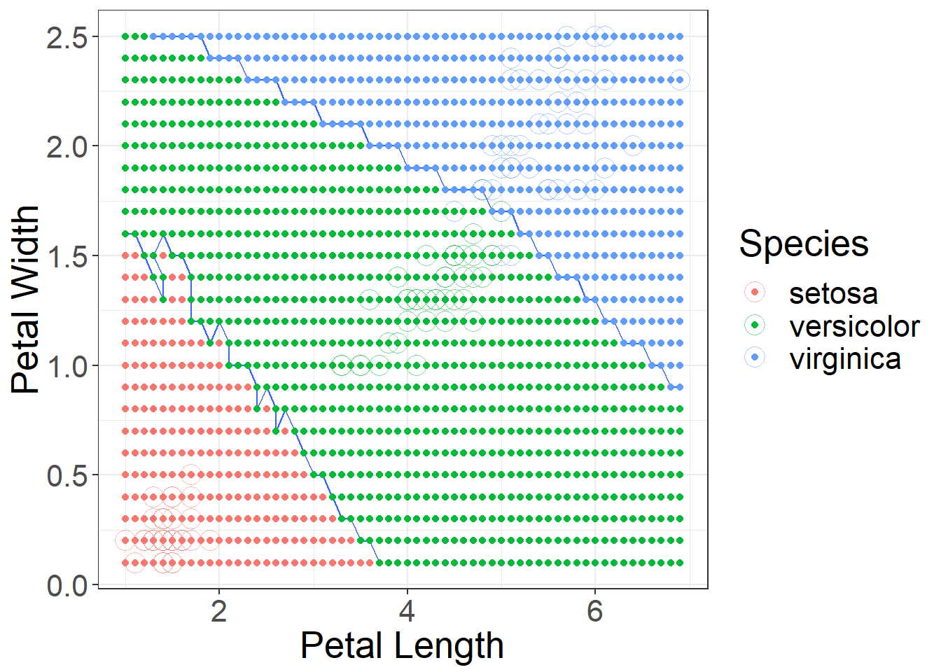
Figure 7: Using k = 10 decision boundaries
Picking the correct features
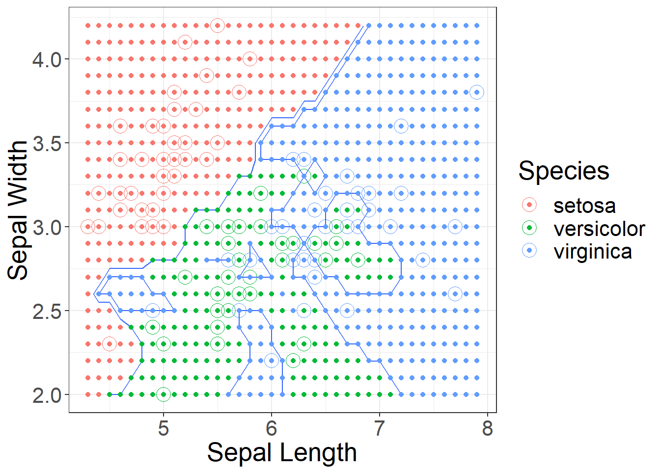
Figure 8: Using k = 1 decision boundaries for Sepal Length and Width
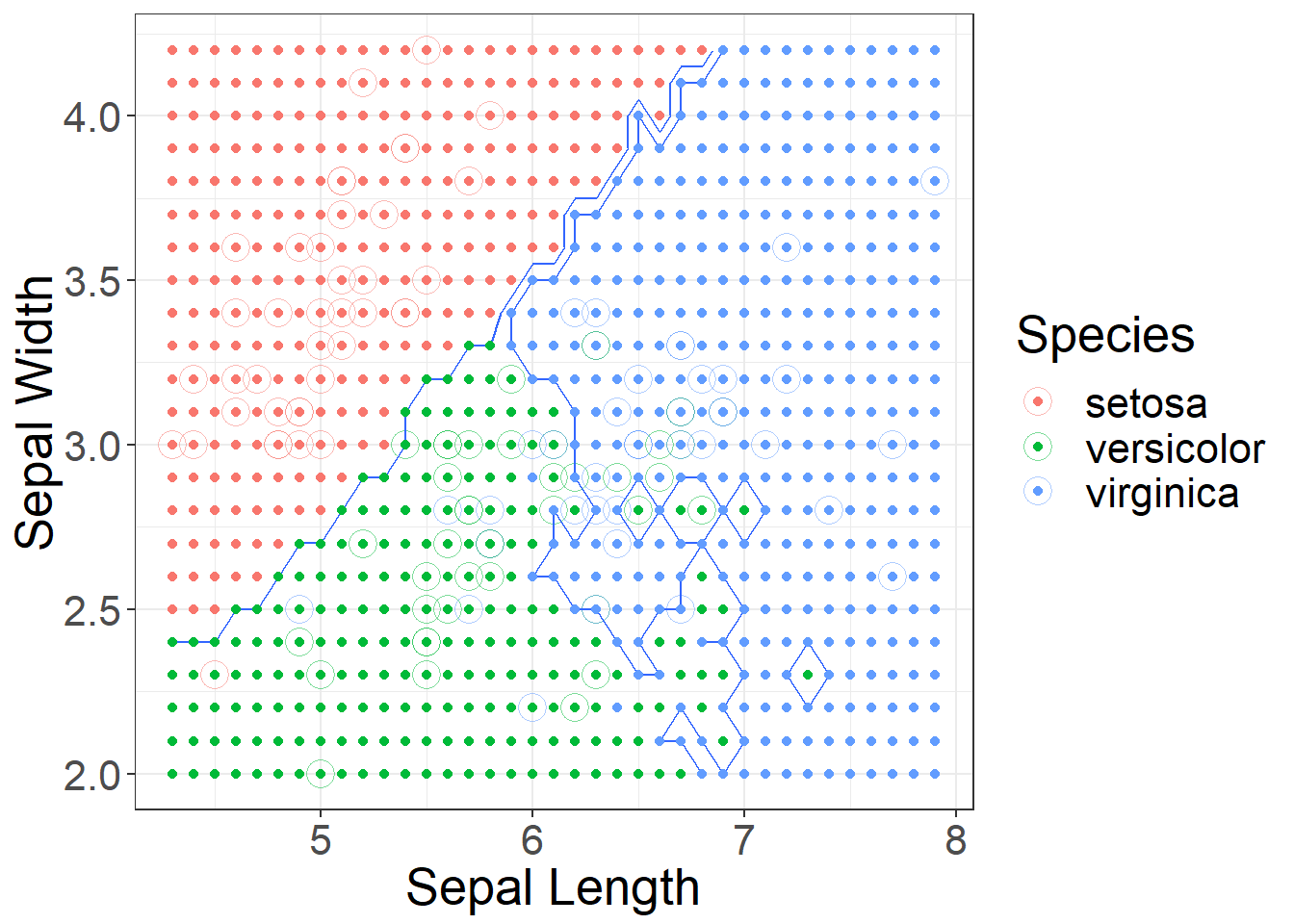
Figure 9: Using k = 10 decision boundaries for Sepal Length and Width
Scaling
Scaling your data is an important process when using KNN. For example we could measure people’s height in meters and weight in kilograms. If we looked at the following people using KNN we would say person 1 and 3 are closer than 1 and 2.
| Height (ft) | Weight (lbs) | |
|---|---|---|
| 1 | 6.25 | 200 |
| 2 | 6.25 | 195 |
| 3 | 5 | 200 |
Person 1 and 2 would have a distance of 5, and Person 1 and 3 would have a distance of 1.25. This is using a rectilinear distance. The model would say 1 and 3 are more alike, but I think most would argue a 5 lbs difference is less of a difference than a 1 ft 3 in difference in height. ### Categorical features
Another issue is categorical features. For example, if we also knew the person spoke a certain language, such as Spanish, French, or Italian. How could we calculate a straight-line distance. We often assign a dummy variable for each category (1-yes, 0-no). Most packages build this in.
Use the shortcut to take care of these issues
The caret package has the ability to look at several “k” values at one time and pick the best one based on an accuracy measure.
model_knn = train(Species ~ Petal.Length+Petal.Width,
                  data = iris_train,
                  method = "knn",
                  tuneGrid = expand.grid(k = 1:10),
                  trControl = trainControl(method = "cv", number = 10),
                  preProcess = c("center","scale"))
Now to see what it actually did:
model_knn## k-Nearest Neighbors
##
## 120 samples
## 2 predictor
## 3 classes: 'setosa', 'versicolor', 'virginica'
##
## Pre-processing: centered (2), scaled (2)
## Resampling: Cross-Validated (10 fold)
## Summary of sample sizes: 108, 108, 108, 108, 108, 108, ...
## Resampling results across tuning parameters:
##
## k Accuracy Kappa
## 1 0.9583333 0.9375
## 2 0.9333333 0.9000
## 3 0.9583333 0.9375
## 4 0.9583333 0.9375
## 5 0.9583333 0.9375
## 6 0.9583333 0.9375
## 7 0.9583333 0.9375
## 8 0.9583333 0.9375
## 9 0.9583333 0.9375
## 10 0.9583333 0.9375
##
## Accuracy was used to select the optimal model using the largest value.
## The final value used for the model was k = 10.See which k it choose, does it make since?
model_knn$bestTune## k
## 10 10How good does it do on our unseen observations?
predictions = predict(object = model_knn, newdata = iris_test)

confusionMatrix(predictions, iris_test$Species)
## Confusion Matrix and Statistics
##
## Reference
## Prediction setosa versicolor virginica
## setosa 10 0 0
## versicolor 0 10 0
## virginica 0 0 10
##
## Overall Statistics
##
## Accuracy : 1
## 95% CI : (0.8843, 1)
## No Information Rate : 0.3333
## P-Value [Acc > NIR] : 4.857e-15
##
## Kappa : 1
##
## Mcnemar's Test P-Value : NA
##
## Statistics by Class:
##
## Class: setosa Class: versicolor Class: virginica
## Sensitivity 1.0000 1.0000 1.0000
## Specificity 1.0000 1.0000 1.0000
## Pos Pred Value 1.0000 1.0000 1.0000
## Neg Pred Value 1.0000 1.0000 1.0000
## Prevalence 0.3333 0.3333 0.3333
## Detection Rate 0.3333 0.3333 0.3333
## Detection Prevalence 0.3333 0.3333 0.3333
## Balanced Accuracy 1.0000 1.0000 1.0000
Twitter
Facebook
Reddit
LinkedIn
StumbleUpon
Pinterest
Email