
Linear Discriminate Analysis (LDA) is a great classification method. It is simple and interpretable and can perform as well, if not better, than a lot of other fancier models (neural networks that are not interpretable).
Introduction to Linear Discriminant Analysis (LDA)
I will be using the Iris Data set again. First I will split it into a “training” set and a “test” set. The test set will represent the unseen observations.
iris_data = iris%>%
  mutate(id = row_number())

iris_train = iris_data%>%
  sample_frac(.8)

iris_test = iris_data%>%
  anti_join(iris_train, by = "id")
Now I will create an LDA model to classify the species based on the Petal Length and Petal Width.
iris_lda = lda(Species ~ Petal.Length + Petal.Width, data = iris_train)

iris_lda
## Call:
## lda(Species ~ Petal.Length + Petal.Width, data = iris_train)
##
## Prior probabilities of groups:
## setosa versicolor virginica
## 0.3083333 0.3583333 0.3333333
##
## Group means:
## Petal.Length Petal.Width
## setosa 1.470270 0.2513514
## versicolor 4.225581 1.3093023
## virginica 5.482500 2.0350000
##
## Coefficients of linear discriminants:
## LD1 LD2
## Petal.Length 1.461922 -2.312619
## Petal.Width 2.559263 5.289222
##
## Proportion of trace:
## LD1 LD2
## 0.9904 0.0096iris_lda_prediction = predict(iris_lda,iris_test)
table(iris_test$Species,iris_lda_prediction$class)##
## setosa versicolor virginica
## setosa 13 0 0
## versicolor 0 6 1
## virginica 0 1 9When you look at the approximate decision boundaries, you can see the difference between KNN and LDA. LDA decision boundaries will be linear. Figure 1 shows the decision boundaries.
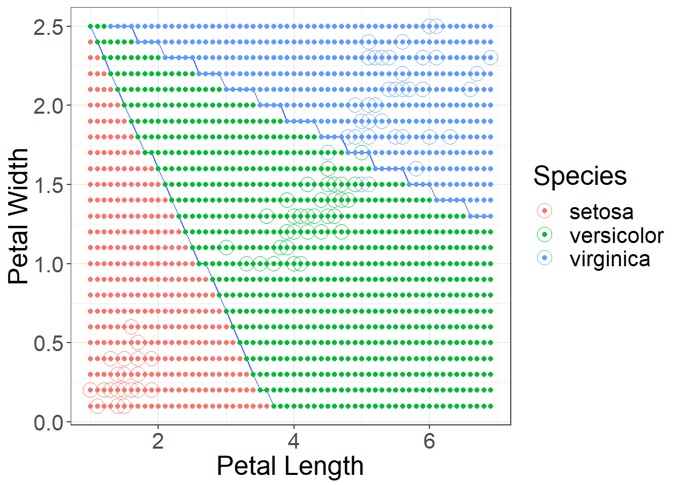
Figure 1: Approximate Decision Boundaries for LDA using Petal Length and Petal Width
Selecting the proper features
iris_lda_sepal = lda(Species ~ Sepal.Length + Sepal.Width,
                     data = iris_train)

iris_lda_sepal
## Call:
## lda(Species ~ Sepal.Length + Sepal.Width, data = iris_train)
##
## Prior probabilities of groups:
## setosa versicolor virginica
## 0.3083333 0.3583333 0.3333333
##
## Group means:
## Sepal.Length Sepal.Width
## setosa 5.024324 3.445946
## versicolor 5.909302 2.758140
## virginica 6.532500 2.980000
##
## Coefficients of linear discriminants:
## LD1 LD2
## Sepal.Length -2.088405 -0.9644933
## Sepal.Width 3.191567 -2.1751277
##
## Proportion of trace:
## LD1 LD2
## 0.9517 0.0483iris_lda_sepal_prediction = predict(iris_lda_sepal,iris_test)
table(iris_test$Species,iris_lda_sepal_prediction$class)##
## setosa versicolor virginica
## setosa 12 1 0
## versicolor 0 5 2
## virginica 0 2 8Recall when using KNN the decision boundaries were not at all linear, now with LDA we have linear boundaries. Figure 2 shows the approximate decision boundaries if we were to use sepal length and sepal width.
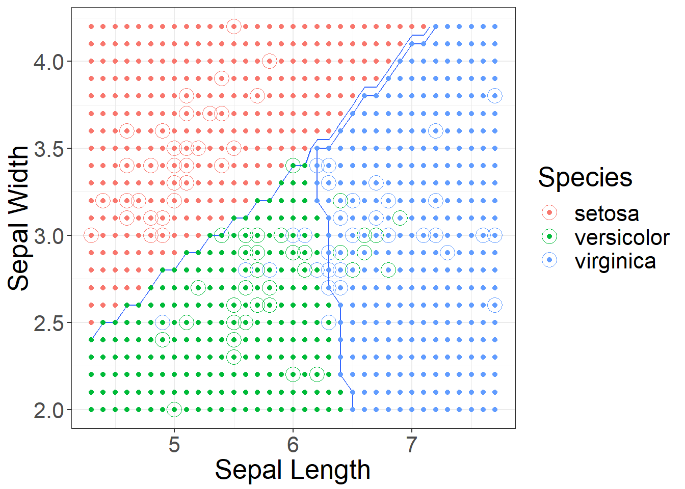
Figure 2: Approximate Decision Boundaries for LDA using Sepal Length and Sepal Width
Using caret for LDA
fitControl = trainControl(
  method = "cv",
  number = 10)

lda_fit = train(Species~Petal.Length+Petal.Width,
                data = iris_train,
                method = "lda",
                trControl = fitControl)

lda_fit
## Linear Discriminant Analysis
##
## 120 samples
## 2 predictor
## 3 classes: 'setosa', 'versicolor', 'virginica'
##
## No pre-processing
## Resampling: Cross-Validated (10 fold)
## Summary of sample sizes: 108, 109, 107, 108, 109, 108, ...
## Resampling results:
##
## Accuracy Kappa
## 0.9651515 0.9475lda_fit$finalModel## Call:
## lda(x, grouping = y)
##
## Prior probabilities of groups:
## setosa versicolor virginica
## 0.3083333 0.3583333 0.3333333
##
## Group means:
## Petal.Length Petal.Width
## setosa 1.470270 0.2513514
## versicolor 4.225581 1.3093023
## virginica 5.482500 2.0350000
##
## Coefficients of linear discriminants:
## LD1 LD2
## Petal.Length 1.461922 -2.312619
## Petal.Width 2.559263 5.289222
##
## Proportion of trace:
## LD1 LD2
## 0.9904 0.0096
Twitter
Facebook
Reddit
LinkedIn
StumbleUpon
Pinterest
Email