
Logistic regression is the last method I shared with the Army unit. I believe logistic regression is an excellent classification model. You are limited to two outcomes, but it is interpretable.
Logistic Regression
This example uses the titanic survival data to walk through a logistic regression example. The question is, what increases your probability of survival.
titanic = titanic::titanic_trainExploring the Data
Figures 1, 2, and 3 graphically depict the relationship between possible explanatory variables and the response variable (surviving). We are looking for a easily identifiable split between surviving and not surviving. Normally you will not be lucky enough to have a clean split, but some are more separated than others.
titanic%>%
  ggplot(aes(x = Age, y = Survived))+
  geom_jitter(height = .1, width = .1)+
  scale_y_continuous(limits = c(-0.1,1.1), breaks = c(0,1))+
  labs(x = "Age (years)", y = "Survived (1 = yes, 0 = no)")
## Warning: Removed 177 rows containing missing values (geom_point).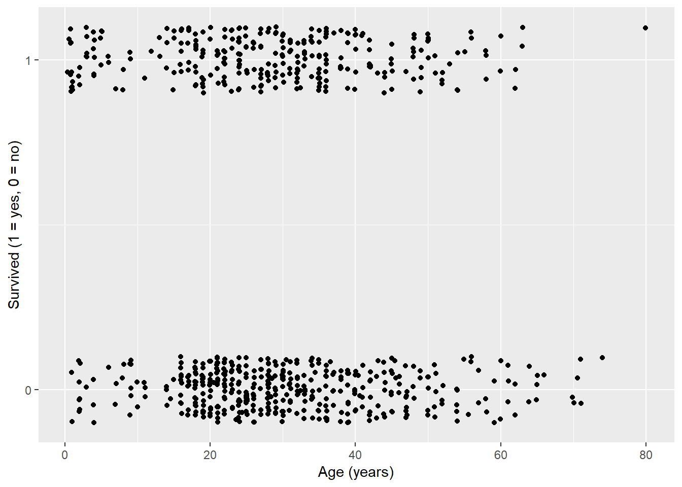
Figure 1: Age versus Surviving
titanic%>%
  ggplot(aes(x = Pclass, y = Survived))+
  geom_jitter(height = 0.1, width = 0.1)+
  scale_y_continuous(limits = c(-0.1,1.1), breaks = c(0,1))+
  labs(x = "Passenger Class", y = "Survived (1 = yes, 0 = no)")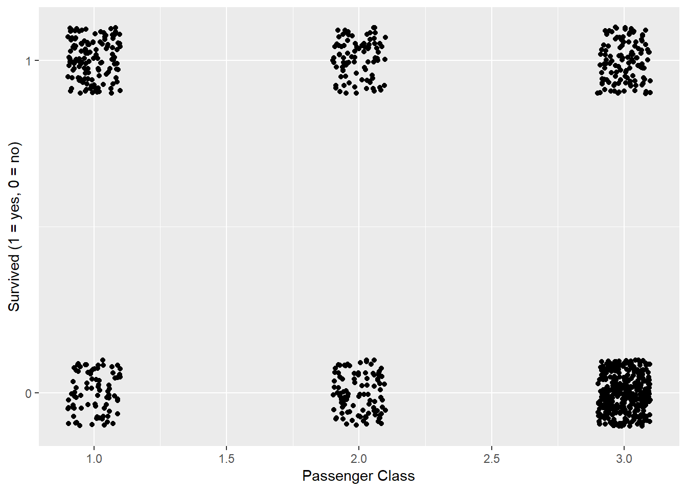
Figure 2: Passenger Class versus Surviving
titanic%>%
  ggplot(aes(x = Sex, y = Survived))+
  geom_jitter(height = 0.1, width = 0.1)+
  scale_y_continuous(limits = c(-0.1,1.1), breaks = c(0,1))+
  labs(x = "Passenger Class", y = "Survived (1 = yes, 0 = no)")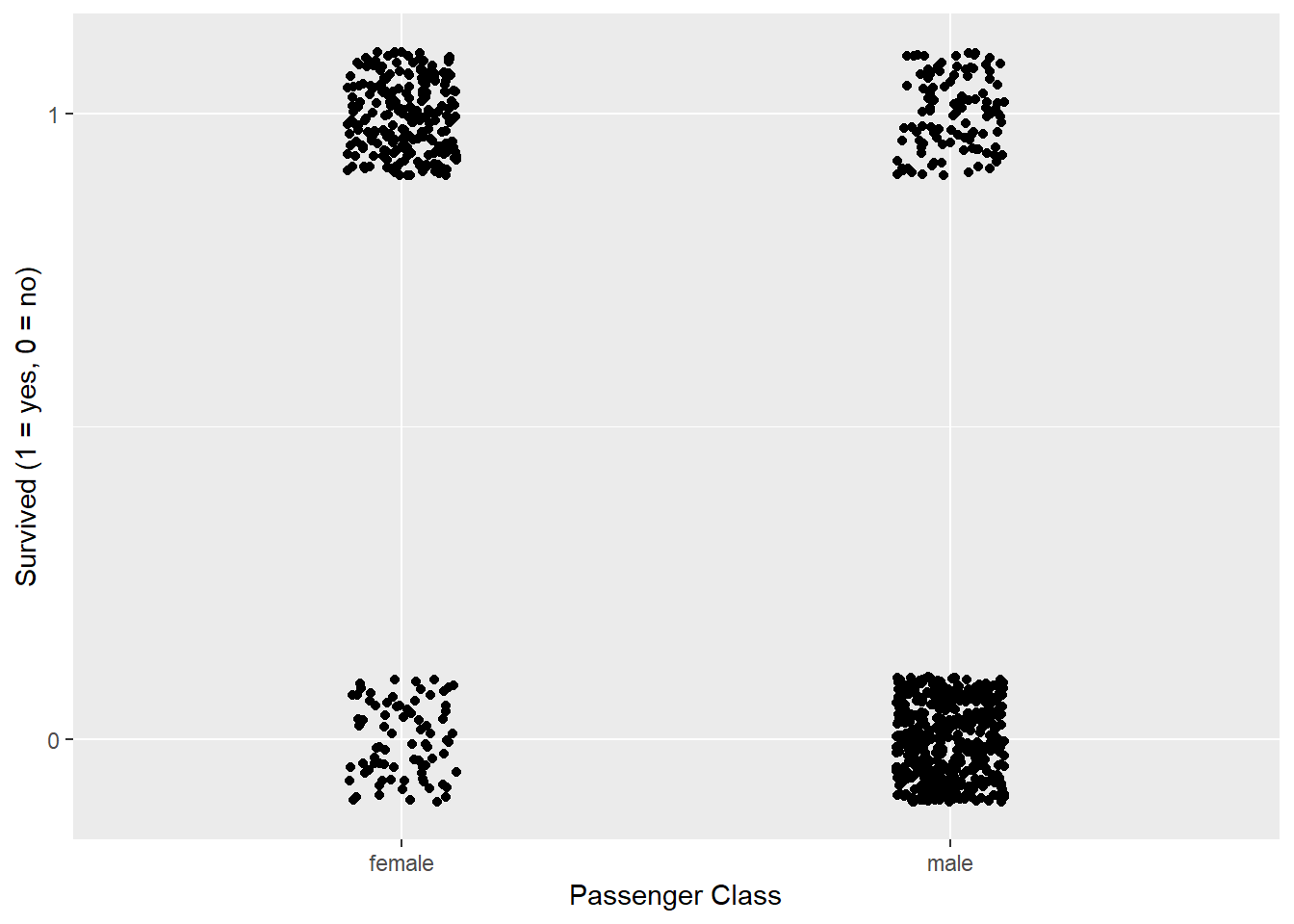
Figure 3: Gender versus Surviving
Making a logistic model using gender as the explanatory varaible
A logistic model returns a probability of having a success (surviving). The coefficients in the model of very little meaning. We are often concerned with an odds ratio. An odds ratio has a real interpretation. Example a team is 2 times more likely to win. We will use gender to explain how to interpret the logistic regression model.
gender_model = glm(Survived ~ Sex, data = titanic, family = binomial)

summary(gender_model)
##
## Call:
## glm(formula = Survived ~ Sex, family = binomial, data = titanic)
##
## Deviance Residuals:
## Min 1Q Median 3Q Max
## -1.6462 -0.6471 -0.6471 0.7725 1.8256
##
## Coefficients:
## Estimate Std. Error z value Pr(>|z|)
## (Intercept) 1.0566 0.1290 8.191 2.58e-16 ***
## Sexmale -2.5137 0.1672 -15.036 < 2e-16 ***
## ---
## Signif. codes: 0 '***' 0.001 '**' 0.01 '*' 0.05 '.' 0.1 ' ' 1
##
## (Dispersion parameter for binomial family taken to be 1)
##
## Null deviance: 1186.7 on 890 degrees of freedom
## Residual deviance: 917.8 on 889 degrees of freedom
## AIC: 921.8
##
## Number of Fisher Scoring iterations: 4If I were to write out the model mathematically it would look like this.
\[p(x) = 1.0566 - 2.5137*Sex\] \[\text{sex}=1\text{ if male}, 0\text{ if female}\] \[p(x) = \text{ The probability of surviving}\]
The value -2.5137 is the log-odds which has no common meaning. If we manipulate it by \(e^{\beta_1}\) we get the odds ratio which has a commonly understood meaning. In this case we get the following odds ratio
exp(gender_model$coefficients[2])## Sexmale
## 0.08096732The odds ratio is 0.081. Because the explanatory variable is categorical, if you are male you are 0.081 times more likely to survive than a female. This is still a little weird to explain, but it does mean you are much more likely to die if you are male. We can switch the survival coding to make it a little more interpretable.
gender_model_flip = glm(Survived ~ Sex, data = titanic%>%
                          mutate(Survived = ifelse(Survived==1,0,1)), family = binomial)

summary(gender_model_flip)
##
## Call:
## glm(formula = Survived ~ Sex, family = binomial, data = titanic %>%
## mutate(Survived = ifelse(Survived == 1, 0, 1)))
##
## Deviance Residuals:
## Min 1Q Median 3Q Max
## -1.8256 -0.7725 0.6471 0.6471 1.6462
##
## Coefficients:
## Estimate Std. Error z value Pr(>|z|)
## (Intercept) -1.0566 0.1290 -8.191 2.58e-16 ***
## Sexmale 2.5137 0.1672 15.036 < 2e-16 ***
## ---
## Signif. codes: 0 '***' 0.001 '**' 0.01 '*' 0.05 '.' 0.1 ' ' 1
##
## (Dispersion parameter for binomial family taken to be 1)
##
## Null deviance: 1186.7 on 890 degrees of freedom
## Residual deviance: 917.8 on 889 degrees of freedom
## AIC: 921.8
##
## Number of Fisher Scoring iterations: 4exp(gender_model_flip$coefficients[2])## Sexmale
## 12.35066In this case, we would say that you are 12.35 times more likely to die if you are male than female.
How well does our model do?
titanic_pred = titanic%>%
  mutate(prediction_probs = predict(gender_model, titanic, type = "response"))%>%
  mutate(pred_survival = ifelse(prediction_probs>=.5,1,0))

table(titanic_pred$Survived, titanic_pred$pred_survival)
##
## 0 1
## 0 468 81
## 1 109 233With this simple model we correctly identified 78.7% of the outcomes, but is this good. A naive approach would be that I state everyone survived. In this data set that would result in being correct 61.6% of the time.
Good I do better with more predictors?
fitControl = trainControl(
  method = "cv",
  number = 10,
  savePredictions = TRUE)

titanic_model = train(as.factor(Survived) ~ Sex,
                      data = titanic,
                      method = "glm",
                      family = binomial(),
                      trControl = fitControl,
na.action = na.pass)titanic_model## Generalized Linear Model
##
## 891 samples
## 1 predictor
## 2 classes: '0', '1'
##
## No pre-processing
## Resampling: Cross-Validated (10 fold)
## Summary of sample sizes: 802, 801, 801, 802, 802, 802, ...
## Resampling results:
##
## Accuracy Kappa
## 0.7867348 0.5421422summary(titanic_model)##
## Call:
## NULL
##
## Deviance Residuals:
## Min 1Q Median 3Q Max
## -1.6462 -0.6471 -0.6471 0.7725 1.8256
##
## Coefficients:
## Estimate Std. Error z value Pr(>|z|)
## (Intercept) 1.0566 0.1290 8.191 2.58e-16 ***
## Sexmale -2.5137 0.1672 -15.036 < 2e-16 ***
## ---
## Signif. codes: 0 '***' 0.001 '**' 0.01 '*' 0.05 '.' 0.1 ' ' 1
##
## (Dispersion parameter for binomial family taken to be 1)
##
## Null deviance: 1186.7 on 890 degrees of freedom
## Residual deviance: 917.8 on 889 degrees of freedom
## AIC: 921.8
##
## Number of Fisher Scoring iterations: 4titanic_model = train(as.factor(Survived) ~ Sex + Age,
data = titanic,
method = "glm",
family = binomial(),
trControl = fitControl,
na.action = na.pass)titanic_model## Generalized Linear Model
##
## 891 samples
## 2 predictor
## 2 classes: '0', '1'
##
## No pre-processing
## Resampling: Cross-Validated (10 fold)
## Summary of sample sizes: 803, 801, 801, 802, 802, 802, ...
## Resampling results:
##
## Accuracy Kappa
## 0.7794228 0.5356102summary(titanic_model)##
## Call:
## NULL
##
## Deviance Residuals:
## Min 1Q Median 3Q Max
## -1.7405 -0.6885 -0.6558 0.7533 1.8989
##
## Coefficients:
## Estimate Std. Error z value Pr(>|z|)
## (Intercept) 1.277273 0.230169 5.549 2.87e-08 ***
## Sexmale -2.465920 0.185384 -13.302 < 2e-16 ***
## Age -0.005426 0.006310 -0.860 0.39
## ---
## Signif. codes: 0 '***' 0.001 '**' 0.01 '*' 0.05 '.' 0.1 ' ' 1
##
## (Dispersion parameter for binomial family taken to be 1)
##
## Null deviance: 964.52 on 713 degrees of freedom
## Residual deviance: 749.96 on 711 degrees of freedom
## (177 observations deleted due to missingness)
## AIC: 755.96
##
## Number of Fisher Scoring iterations: 4titanic_model = train(as.factor(Survived) ~ Sex + Age + Pclass,
data = titanic,
method = "glm",
family = binomial(),
trControl = fitControl,
na.action = na.pass)titanic_model## Generalized Linear Model
##
## 891 samples
## 3 predictor
## 2 classes: '0', '1'
##
## No pre-processing
## Resampling: Cross-Validated (10 fold)
## Summary of sample sizes: 802, 803, 801, 802, 802, 802, ...
## Resampling results:
##
## Accuracy Kappa
## 0.79171 0.5641345summary(titanic_model)##
## Call:
## NULL
##
## Deviance Residuals:
## Min 1Q Median 3Q Max
## -2.7270 -0.6799 -0.3947 0.6483 2.4668
##
## Coefficients:
## Estimate Std. Error z value Pr(>|z|)
## (Intercept) 5.056006 0.502128 10.069 < 2e-16 ***
## Sexmale -2.522131 0.207283 -12.168 < 2e-16 ***
## Age -0.036929 0.007628 -4.841 1.29e-06 ***
## Pclass -1.288545 0.139259 -9.253 < 2e-16 ***
## ---
## Signif. codes: 0 '***' 0.001 '**' 0.01 '*' 0.05 '.' 0.1 ' ' 1
##
## (Dispersion parameter for binomial family taken to be 1)
##
## Null deviance: 964.52 on 713 degrees of freedom
## Residual deviance: 647.29 on 710 degrees of freedom
## (177 observations deleted due to missingness)
## AIC: 655.29
##
## Number of Fisher Scoring iterations: 5I can now compare the accuracy measures for each of the models and decide on the optimal model.
confusionMatrix(titanic_model)## Cross-Validated (10 fold) Confusion Matrix
##
## (entries are percentual average cell counts across resamples)
##
## Reference
## Prediction 0 1
## 0 50.0 11.5
## 1 9.4 29.1
##
## Accuracy (average) : 0.7913Is your model just guessing
ROC can be seen as a grade. A 1 is an A+, a .5 is an F, or really your model is just guessing.
Here are two ways to look at it, one visual and one with the numeric calculation.
titanic_predictions = predict(gender_model, titanic,
                              type = "response")

colAUC(titanic_predictions,titanic$Survived, plotROC = T)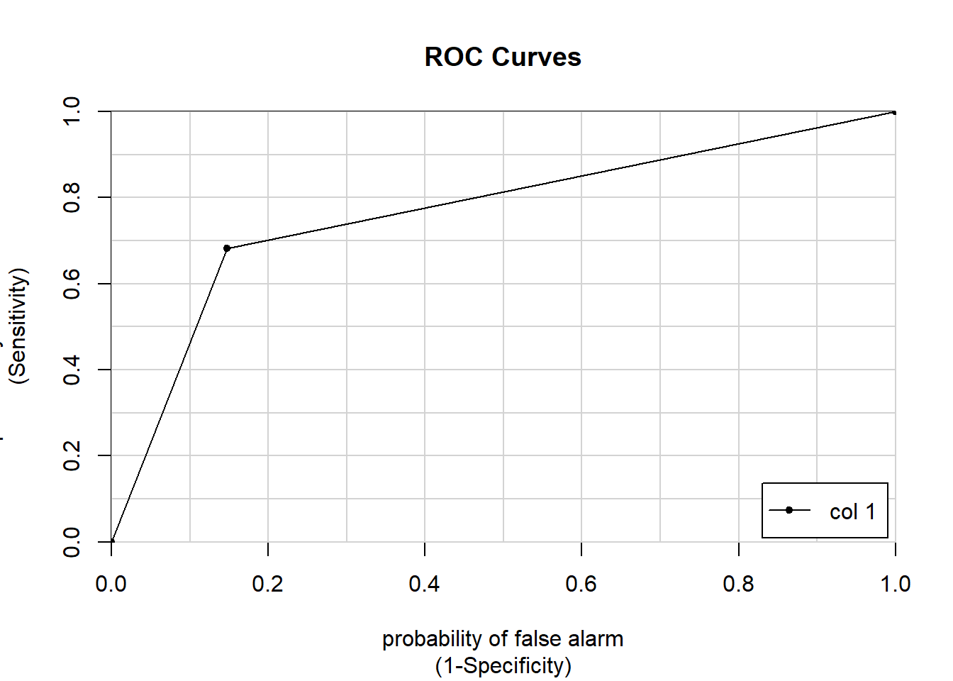
##              [,1]
## 0 vs. 1 0.7668728
fitControl = trainControl(
method = "cv",
number = 10,
summaryFunction = twoClassSummary,
classProbs = TRUE, # IMPORTANT!
verboseIter = TRUE)
titanic_model = train(make.names(Survived) ~ Sex,
data = titanic,
method = "glm",
trControl = fitControl,
na.action = na.pass)## Warning in train.default(x, y, weights = w, ...): The metric "Accuracy" was
## not in the result set. ROC will be used instead.## + Fold01: parameter=none
## - Fold01: parameter=none
## + Fold02: parameter=none
## - Fold02: parameter=none
## + Fold03: parameter=none
## - Fold03: parameter=none
## + Fold04: parameter=none
## - Fold04: parameter=none
## + Fold05: parameter=none
## - Fold05: parameter=none
## + Fold06: parameter=none
## - Fold06: parameter=none
## + Fold07: parameter=none
## - Fold07: parameter=none
## + Fold08: parameter=none
## - Fold08: parameter=none
## + Fold09: parameter=none
## - Fold09: parameter=none
## + Fold10: parameter=none
## - Fold10: parameter=none
## Aggregating results
## Fitting final model on full training settitanic_model## Generalized Linear Model
##
## 891 samples
## 1 predictor
## 2 classes: 'X0', 'X1'
##
## No pre-processing
## Resampling: Cross-Validated (10 fold)
## Summary of sample sizes: 801, 802, 802, 802, 802, 802, ...
## Resampling results:
##
## ROC Sens Spec
## 0.7670356 0.8523906 0.6816807Age is more continuous which will give a better visualization of the ROC curve
age_model = glm(Survived ~ Age, data = titanic, family = binomial)

summary(age_model)
##
## Call:
## glm(formula = Survived ~ Age, family = binomial, data = titanic)
##
## Deviance Residuals:
## Min 1Q Median 3Q Max
## -1.1488 -1.0361 -0.9544 1.3159 1.5908
##
## Coefficients:
## Estimate Std. Error z value Pr(>|z|)
## (Intercept) -0.05672 0.17358 -0.327 0.7438
## Age -0.01096 0.00533 -2.057 0.0397 *
## ---
## Signif. codes: 0 '***' 0.001 '**' 0.01 '*' 0.05 '.' 0.1 ' ' 1
##
## (Dispersion parameter for binomial family taken to be 1)
##
## Null deviance: 964.52 on 713 degrees of freedom
## Residual deviance: 960.23 on 712 degrees of freedom
## (177 observations deleted due to missingness)
## AIC: 964.23
##
## Number of Fisher Scoring iterations: 4titanic_predictions = predict(age_model, titanic,
type = "response")
colAUC(titanic_predictions,titanic$Survived, plotROC = T)## Warning in matrix(rep(idx, nL), nR, nL): data length [1428] is not a sub-
## multiple or multiple of the number of rows [891]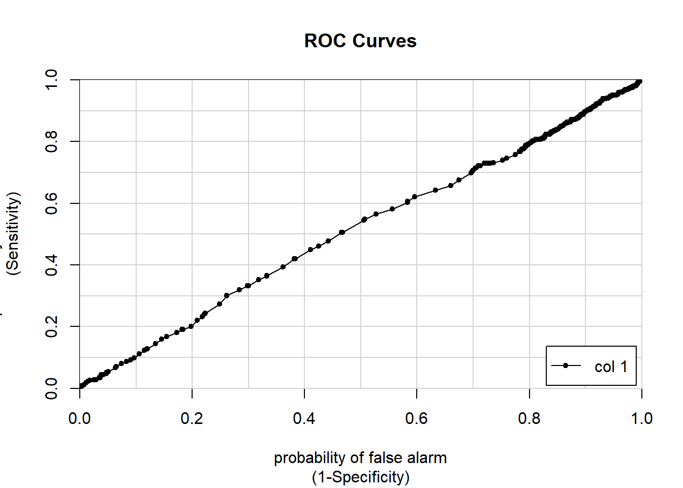
##              [,1]
## 0 vs. 1 0.5130549
Twitter
Facebook
Reddit
LinkedIn
StumbleUpon
Pinterest
Email